Contact Tracing Example
Contact tracing and isolation can be an effective way to stop or slow the spread of an outbreak. In this post, we’ll examine a method for determining potentially infected contacts based on a provided trace.

Overview
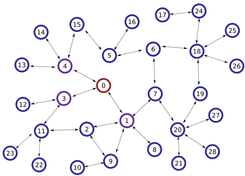
The image above illustrates a hypothetical scenario where patient zero has several contacts, who, in turn, each have several contacts of their own, and so on. This branching tree of contacts creates our contact trace, an adjacency list of the contacts of each person. In this post, we explore an efficient method for determining the exposure risk to this population based on proximity to patient zero. To carry this out, we create a contact matrix to efficiently determine direct contacts, contacts once removed, and contacts twice removed. The code and sample data for this post is available here.
Exposure Risk Levels
In this example, each person’s risk is deteremined according to their proximity to patient zero. Direct contacts are at the highest risk, followed by contacts once removed (the contacts of the direct contacts), followed by contacts twice removed. In this model, direct contacts will be asked to quarantine, contacts once removed will be asked self-isolate to minimize exposure, and contacts twice removed will be given extra testing.
Determinining Contact Levels
An effective way to quickly determine the contact level for each person is to transform the provided contact adjacency list into a contact adjacency matrix. The contact matrix, as we’ll see below, will provide useful properties for quickly determining not only the degree of separation between a person and patient zero, but also the number of potential paths of infection.
Building a Contact Matrix
The code below transforms the provided adjacency list into a contact matrix:
contact_matrix = np.zeros((contact_count,contact_count),dtype=int)
for k in contact_trace:
    for v in contact_trace[k]:
        contact_matrix[k][v] = 1
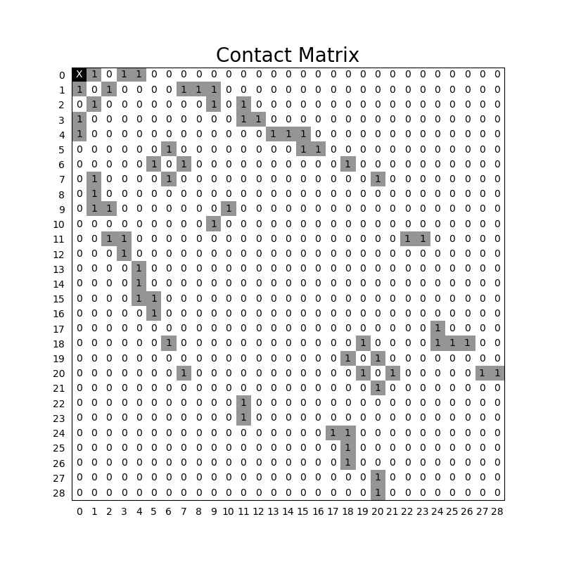
Here is a visualization of the contact matrix using Matplotlib:

This matrix shows direct contacts between each person in the contact trace, if two people have been in contact, their will be a ‘1’ at their intersection, otherwise there will be a ‘0’ if they haven’t had direct contact. In this example all contacts are bi-directional, meaning that if person A has been in contact with person B then person B will have been in contact with person A. For this reason, the matrix is mirrored along its trace.
Contact Tracing
We can use the matrix we created to quickly calculate the degree of separation between each person and patient zero. In each subsection, we’ll examine the methodology.
Level 1 – Direct Contacts: Quarantine
 The contact matrix tells us how many paths of length one exist between each person. The first degree of separation (direct contacts) can be seen by simply examining the row of the matrix corresponding to patient zero since everyone in this row had direct contact with patient zero.
Level 2 – Contacts once removed: Isolation
 As you may recall from math class, squaring the contact matrix tells us how many paths of length two exist between each person. Once again, examining the row corresponding to patient zero reveals our contacts once removed.
Level 3 – Contacts twice removed: Monitoring
 Similarly, cubing the contact matrix tells us how many paths of length three exist between each person. Again, examining the row corresponding to patient zero, we find many new individuals who should be tested and also see some of our previously detected contacts since there are also paths of length three between them and patient zero.
Conclusion
Matrix-based contact tracing provides a simple method for understanding how contact tracing could work in practice and could provide a useful tool in slowing the spread of an outbreak. It could also be used to slow the spread of less threatening existing diseases, potentially lowering their effective reproductive rate below one meaning that some diseases like the flu could become less of a problem in the future if this technique is used effectively.