Data Wrangling with PostgreSQL
Wrangling raw data into well normalized, efficiently queryable tables in PostgreSQL can be challenging, especially for those with limited prior SQL exposure. In this tutorial, I’ve created a step by step guide to walk you through the process of munging and normalizing data about famous people from a practice data set.
Before starting, please download and import this practice database into PostgreSQL.
Eliminating Anomalies
Before we can begin organizing our raw data up into separate normalized tables, we will need to eliminate the anomalies in our data. For example, in the nationality field, “Dutch” and “Holland” both refer to the same nationality, but, if we want to search for everyone from the Netherlands, we would need to include both terms separately. Repairing these types of issues will require some wrangling as there are non-normalized duplicates in both the occupation and nationality fields.
To update a table value in PostgreSQL, use the follow command structure:
UPDATE <table name>
SET <column name> = <new value>
<condition clause(s)>
Example:
UPDATE raw_data
SET nationality = 'Netherlands'
WHERE nationality = 'Holland'
OR nationality = 'Dutch'
As an exercise, continue the normalization process on your own. To check whether you have successfully removed all anomalies, use a query with the following structure:
SELECT DISTINCT <column name> FROM <table name> ORDER BY <column name>Example:
SELECT DISTINCT occupation FROM raw_data ORDER BY occupationFor larger lists, you might need to bring in a tool like Open Refine, but for this tutorial, you should be able to verify that each field is normalized by eye.
For the purposes of this tutorial it is not critical the you update every nationality to reflect the appropriate demonym, but simply that you make sure that every nationality and occupation in the the raw_data table is represented consistently.
Modeling Ancillary Data Tables
After all of the anomalies are removed, we can create new tables to organize our data. Before creating the new tables, it might be helpful to think in terms of classes (generalizations) and instances (specific examples) where the table structure represents a model consisting of an identifier and properties or attributes (a generalization) and each row represents an instantiation (a specific example) of that model.
As an example, let’s take a look at the first five rows of our raw_data table using the following query:
SELECT * FROM raw_data LIMIT 5Here are our results:
| person | occupation | nationality | estimated_iq_score |
|---|---|---|---|
| Abraham Lincoln | politician | USA | 128 |
| Marilyn vos Savant | writer | USA | 186 |
| Rene Descartes | philosopher | France | 185 |
| Thomas Chatterton | writer | England | 180 |
| Sofia Kovalevskaya | scientist | Russia | 170 |
The fields in our raw_data table are all attributes of a person, so it makes sense to make create a person table with normalized attributes.
Before we create a “person” table, however, the raw_data table has two columns that look like good candidates for further normalization as ancillary tables:
| nationality |
| occupation |
The reason that we want to factor these attributes out into separate tables is that, when properly normalized, we can make attribute updates in a single place as opposed to applying updates across the entirety one or more tables.
For example, imagine we wanted to update the nationality attribute labeled ‘USA’ to become ‘American’. In our non-normalized raw data, we would need to use the following statement:
UPDATE raw_data
SET nationality = 'American'
WHERE nationality = 'USA'
Which would inefficiently act on 31 records as opposed to a single row if our data were properly normalized. Furthermore, in more complicated databases, there could be multiple tables that use the nationality attribute which would also need to be updated.
Each of your ancillary tables should contain fields:
| Field Name | Type | Constraint | Reference |
|---|---|---|---|
| id | serial | primary key | |
| name | character varying |
Once these tables are created, you can use the following command structure to populate them from you raw_data table:
DROP SEQUENCE IF EXISTS <sequence name>;
CREATE SEQUENCE <sequence name> START 1;
INSERT INTO <destination table>
SELECT NEXTVAL('<sequence name>'),<column name> FROM (SELECT DISTINCT <column name> FROM <origin table>) <subquery alias>
Example:
DROP SEQUENCE IF EXISTS serial;
CREATE SEQUENCE serial START 1;
INSERT INTO nationality
SELECT NEXTVAL('serial'),nationality FROM (SELECT DISTINCT nationality FROM raw_data) t;
Modeling the Person Table
Finally, you will need to create the person table. It should contain the following fields:
| Field Name | Type | Constraint | Reference |
|---|---|---|---|
| id | serial | primary key | |
| name | character varying | ||
| nationality_id | integer | foreign key | nationality |
| occupation_id | integer | foreign key | occupation |
| estimated_iq_score | integer |
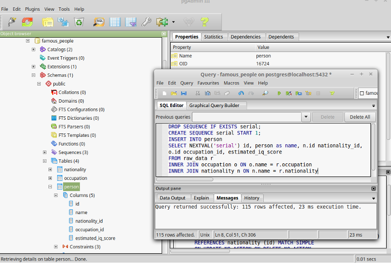
Once the “person” table is created you can use the following command to populate its records:
DROP SEQUENCE IF EXISTS serial;
CREATE SEQUENCE serial START 1;
INSERT INTO person
SELECT NEXTVAL('serial') id, person as name, n.id nationality_id, o.id occupation_id, estimated_iq_score
FROM raw_data r
INNER JOIN occupation o ON o.name = r.occupation
INNER JOIN nationality n ON n.name = r.nationality
Query the “person” table. You should have 115 normalized records.
Conclusion
Congratulations! This completes the tutorial. In the next tutorial, we will use this database for exercises to practice concepts in querying.